Bellman-Ford
The Bellman-Ford algorithm is a graph algorithm used for finding the shortest paths from a single source vertex to all other vertices in a weighted graph, even if the graph contains negative weight edges. It works as follows: 1. Initialization: Set the distance to the source vertex to zero and the distances to all other vertices to infinity. 2. Relaxation: For each edge in the graph, update the distance to the destination vertex if the distance to the source vertex plus the edge weight is less than the current distance to the destination vertex. Repeat this process for a total of |V| - 1 times, where |V| is the number of vertices in the graph. 3. Negative Cycle Detection: Check for negative weight cycles by iterating through all edges once more. If any distance can be updated, a negative weight cycle exists in the graph. The Bellman-Ford algorithm is slower than Dijkstras algorithm, with a time complexity of O(V * E), but it is more versatile as it can handle graphs with negative weight edges.
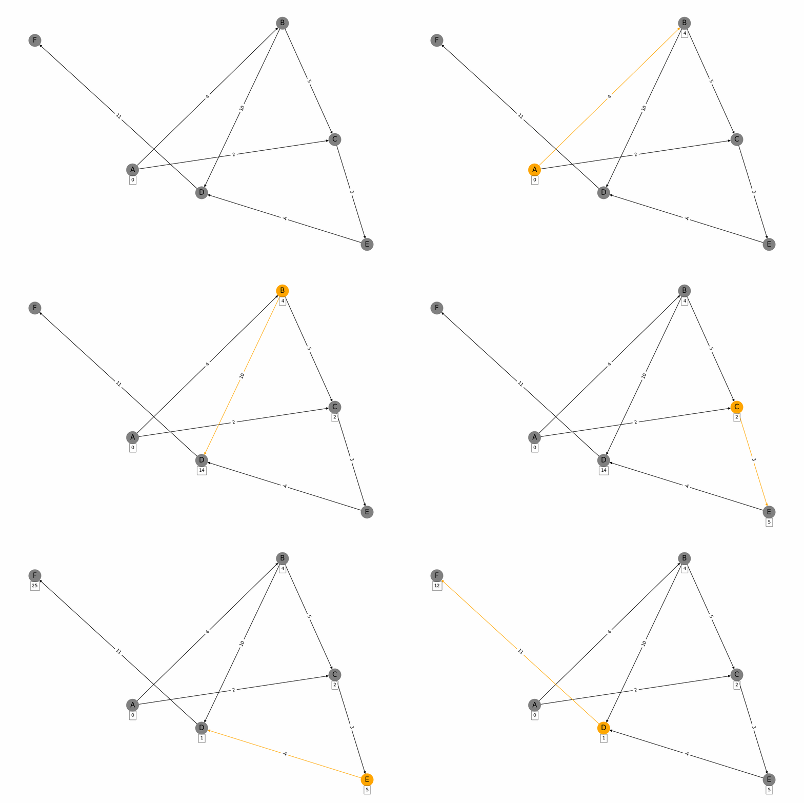
import networkx as nx
import matplotlib.pyplot as plt
from PIL import Image, ImageDraw
import os
# Create a weighted graph
G = nx.DiGraph()
# Add nodes and weighted edges
edges = [
    ('A', 'B', 4), ('A', 'C', 2),
    ('B', 'C', 5), ('B', 'D', 10),
    ('C', 'E', 3), ('D', 'F', 11),
    ('E', 'D', -4)  # Negative weight for demonstration
]
for edge in edges:
    G.add_edge(edge[0], edge[1], weight=edge[2])
# Function to visualize the graph at each step
def draw_graph(G, pos, node_colors, edge_colors, discovered_weights, filename):
    plt.figure(figsize=(12, 8))  # Increase figure size
    nx.draw(G, pos, with_labels=True, node_color=node_colors, edge_color=edge_colors, node_size=700, font_size=15)
    edge_labels = nx.get_edge_attributes(G, 'weight')
    nx.draw_networkx_edge_labels(G, pos, edge_labels=edge_labels)
    # Annotate nodes with discovered weights
    for node, weight in discovered_weights.items():
        plt.text(pos[node][0], pos[node][1]-0.05, s=f'{weight}', bbox=dict(facecolor='white', alpha=0.5), horizontalalignment='center')
    plt.savefig(filename)
    plt.close()

# Bellman-Ford algorithm visualization
def bellman_ford_visualization(G, start):
    pos = nx.random_layout(G)  # Use random_layout for better node spacing
    node_colors = ['grey' for node in G.nodes()]
    edge_colors = ['black' for edge in G.edges()]
    # Create a directory to store the frames
    if not os.path.exists('frames'):
        os.makedirs('frames')
    step = 0
    discovered_weights = {start: 0}
    draw_graph(G, pos, node_colors, edge_colors, discovered_weights, f'frames/step{step}.png')
    nodes = set(G.nodes())
    for _ in range(len(nodes) - 1):
        for u, v, w in G.edges(data=True):
            weight = discovered_weights[u] + w['weight']
            if v not in discovered_weights or weight < discovered_weights[v]:
                discovered_weights[v] = weight
                node_colors = ['orange' if node == u else 'grey' for node in G.nodes()]
                edge_colors = ['orange' if edge[0] == u and edge[1] == v else 'black' for edge in G.edges()]
                step += 1
                draw_graph(G, pos, node_colors, edge_colors, discovered_weights, f'frames/step{step}.png')
    return discovered_weights
# Run the visualization
start_node = 'A'
bellman_ford_visualization(G, start_node)
# Create GIF from frames with slower steps
frames = []
frame_folder = 'frames'
frame_files = sorted([f for f in os.listdir(frame_folder) if f.endswith('.png')], key=lambda x: int(x[4:-4]))
for file in frame_files:
    frames.append(Image.open(os.path.join(frame_folder, file)))
frames[0].save('bellman_ford.gif', save_all=True, append_images=frames[1:], duration=1000, loop=0)
Dijkstra's
Dijkstras algorithm is a popular algorithm used in computer science and graph theory to find the shortest path from a starting node (source) to all other nodes in a weighted graph. Here is a brief summary: 1. Initialization: Start with a graph where each node has a tentative distance. Set the distance of the source node to 0 and all other nodes to infinity. Create a priority queue to keep track of the nodes to be evaluated, initially containing only the source node. 2. Node Selection: Select the node with the smallest tentative distance (initially the source node) and consider all its neighbors. 3. **Distance Update**: For each neighboring node, calculate the distance from the source node to that neighbor through the current node. If this calculated distance is less than the current known distance, update the tentative distance of the neighboring node. 4. **Marking Processed Nodes**: Once all neighbors of the current node have been considered, mark the current node as processed. A processed node will not be checked again. 5. **Repeat**: Repeat the process of selecting the node with the smallest tentative distance, updating distances, and marking nodes as processed until all nodes have been processed or the destination nodes shortest distance is found. 6. **Completion**: The algorithm ends when all nodes have been processed or the smallest distance among the unprocessed nodes is infinity (indicating that the remaining nodes are not reachable from the source). The algorithm guarantees the shortest path in graphs with non-negative weights and has a time complexity of \(O((V + E) \log V)\) using a priority queue, where \(V\) is the number of vertices and \(E\) is the number of edges.
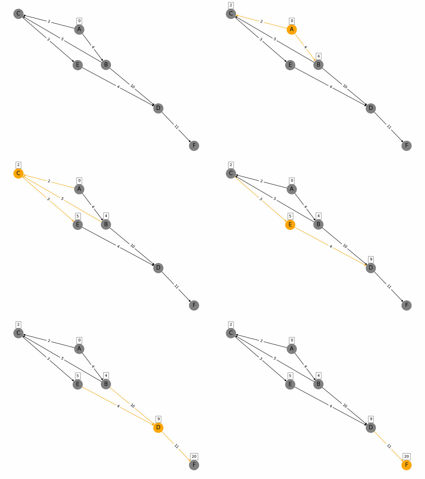
import networkx as nx
import matplotlib.pyplot as plt
from PIL import Image, ImageDraw
import os
# Create a weighted graph
G = nx.DiGraph()
# Add nodes and weighted edges
edges = [
    ('A', 'B', 4), ('A', 'C', 2),
    ('B', 'C', 5), ('B', 'D', 10),
    ('C', 'E', 3), ('D', 'F', 11),
    ('E', 'D', 4)
]
for edge in edges:
    G.add_edge(edge[0], edge[1], weight=edge[2])
# Function to visualize the graph at each step
def draw_graph(G, pos, node_colors, edge_colors, discovered_weights, filename):
    plt.figure(figsize=(8, 6))
    nx.draw(G, pos, with_labels=True, node_color=node_colors, edge_color=edge_colors, node_size=700, font_size=15)
    edge_labels = nx.get_edge_attributes(G, 'weight')
    nx.draw_networkx_edge_labels(G, pos, edge_labels=edge_labels)
    # Annotate nodes with discovered weights
    for node, weight in discovered_weights.items():
        plt.text(pos[node][0], pos[node][1]+0.1, s=f'{weight}', bbox=dict(facecolor='white', alpha=0.5), horizontalalignment='center')
    plt.savefig(filename)
    plt.close()
# Dijkstra's algorithm visualization
def dijkstra_visualization(G, start, target):
    pos = nx.spring_layout(G)
    node_colors = ['grey' for node in G.nodes()]
    edge_colors = ['black' for edge in G.edges()]
    # Create a directory to store the frames
    if not os.path.exists('frames'):
        os.makedirs('frames')
    step = 0
    discovered_weights = {start: 0}
    draw_graph(G, pos, node_colors, edge_colors, discovered_weights, f'frames/step{step}.png')
    visited = {start: 0}
    path = {}
    nodes = set(G.nodes())
    while nodes:
        min_node = None
        for node in nodes:
            if node in visited:
                if min_node is None:
                    min_node = node
                elif visited[node] < visited[min_node]:
                    min_node = node
        if min_node is None:
            break
        nodes.remove(min_node)
        current_weight = visited[min_node]
        for edge in G.edges(min_node, data=True):
            weight = current_weight + edge[2]['weight']
            if edge[1] not in visited or weight < visited[edge[1]]:
                visited[edge[1]] = weight
                path[edge[1]] = min_node
                discovered_weights[edge[1]] = weight
        node_colors = ['orange' if node == min_node else 'grey' for node in G.nodes()]
        edge_colors = ['orange' if edge[0] == min_node or edge[1] == min_node else 'black' for edge in G.edges()]
        step += 1
        draw_graph(G, pos, node_colors, edge_colors, discovered_weights, f'frames/step{step}.png')
    return visited, path
# Run the visualization
start_node = 'A'
target_node = 'F'
dijkstra_visualization(G, start_node, target_node)
# Create GIF from frames with slower steps
frames = []
frame_folder = 'frames'
frame_files = sorted([f for f in os.listdir(frame_folder) if f.endswith('.png')], key=lambda x: int(x[4:-4]))
for file in frame_files:
    frames.append(Image.open(os.path.join(frame_folder, file)))
frames[0].save('graph_traversal.gif', save_all=True, append_images=frames[1:], duration=2000, loop=0)
Bubble Sort
Bubble sort is a simple comparison-based sorting algorithm. It repeatedly steps through the list, compares adjacent elements, and swaps them if they are in the wrong order. This process is repeated until the list is sorted. The algorithm gets its name because smaller elements "bubble" to the top (beginning of the list) while larger elements sink to the bottom (end of the list) with each pass through the list. Key Characteristics: - Time Complexity: O(n²) in the worst and average cases, where n is the number of elements. - Space Complexity: O(1), as it requires only a constant amount of additional space. - Stability: Bubble sort is a stable sort, meaning that it preserves the relative order of equal elements. - Adaptability: It performs best when the list is nearly sorted, as it can detect if the list is already sorted and terminate early. Algorithm Steps: 1. Compare each pair of adjacent elements. 2. Swap them if they are in the wrong order. 3. Repeat the process for all elements in the list. 4. Continue until no swaps are needed, indicating that the list is sorted.

def bubble_sort(arr):
frames = []
n = len(arr)
step = 0
for i in range(n):
    # Traverse through all array elements
    # Last i elements are already in place
    for j in range(0, n-i-1):
        # Traverse the array from 0 to n-i-1
        # Swap if the element found is greater than the next element
        if arr[j] > arr[j+1]:
            arr[j], arr[j+1] = arr[j+1], arr[j]
        # Append current state of array and step count to frames
        frames.append((arr.copy(), step))
        step += 1
return frames
Insertion Sort
Insertion sort is a simple and intuitive comparison-based sorting algorithm. It builds the sorted list one element at a time by repeatedly taking the next unsorted element and inserting it into its correct position within the sorted portion of the list. Key Characteristics: -Time Complexity: O(n²) in the worst and average cases, but O(n) in the best case when the list is already sorted or nearly sorted. -Space Complexity: O(1), as it requires only a constant amount of additional space. -Stability: Insertion sort is a stable sort, meaning that it preserves the relative order of equal elements. -Adaptability: It performs efficiently for small data sets or nearly sorted lists, making it useful for applications where the data is frequently partially sorted. Algorithm Steps: 1. Start with the second element (consider the first element as a sorted sublist of one element). 2. Compare the current element with the elements in the sorted sublist. 3. Shift all elements in the sorted sublist that are greater than the current element one position to the right. 4. Insert the current element into its correct position. 5. Repeat the process for all elements in the list. By the end of the process, the list will be fully sorted.
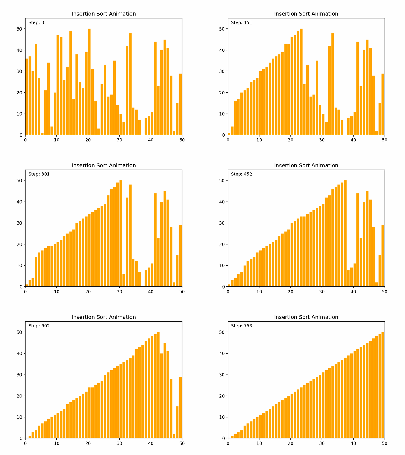
def insertion_sort(arr):
frames = []
step = 0
for i in range(1, len(arr)):
    key = arr[i]
    j = i-1
    # Move elements of arr[0..i-1], that are greater than key,
    # to one position ahead of their current position
    while j >= 0 and key < arr[j]:
        arr[j + 1] = arr[j]
        j -= 1
        # Append current state of array and step count to frames
        frames.append((arr.copy(), step))
        step += 1
    arr[j + 1] = key
    # Append current state of array and step count to frames
    frames.append((arr.copy(), step))
    step += 1
return frames
Selection Sort
Selection sort is a straightforward comparison-based sorting algorithm. It works by repeatedly finding the minimum element from the unsorted portion of the list and swapping it with the first unsorted element, effectively growing the sorted portion of the list one element at a time. Key Characteristics: -Time Complexity: O(n²) for all cases (worst, average, and best), where n is the number of elements. -Space Complexity: O(1), as it requires only a constant amount of additional space. -Stability: Selection sort is not stable, meaning that it does not necessarily preserve the relative order of equal elements. -Adaptability: It is not adaptive, meaning that its performance does not improve with nearly sorted lists. Algorithm Steps: 1. Start with the first element and consider it the minimum. 2. Iterate through the remaining elements to find the smallest element. 3. Swap the smallest element found with the first unsorted element. 4. Move the boundary of the sorted and unsorted portions one element to the right. 5. Repeat the process for the remaining unsorted elements. By the end of the process, the entire list will be sorted.
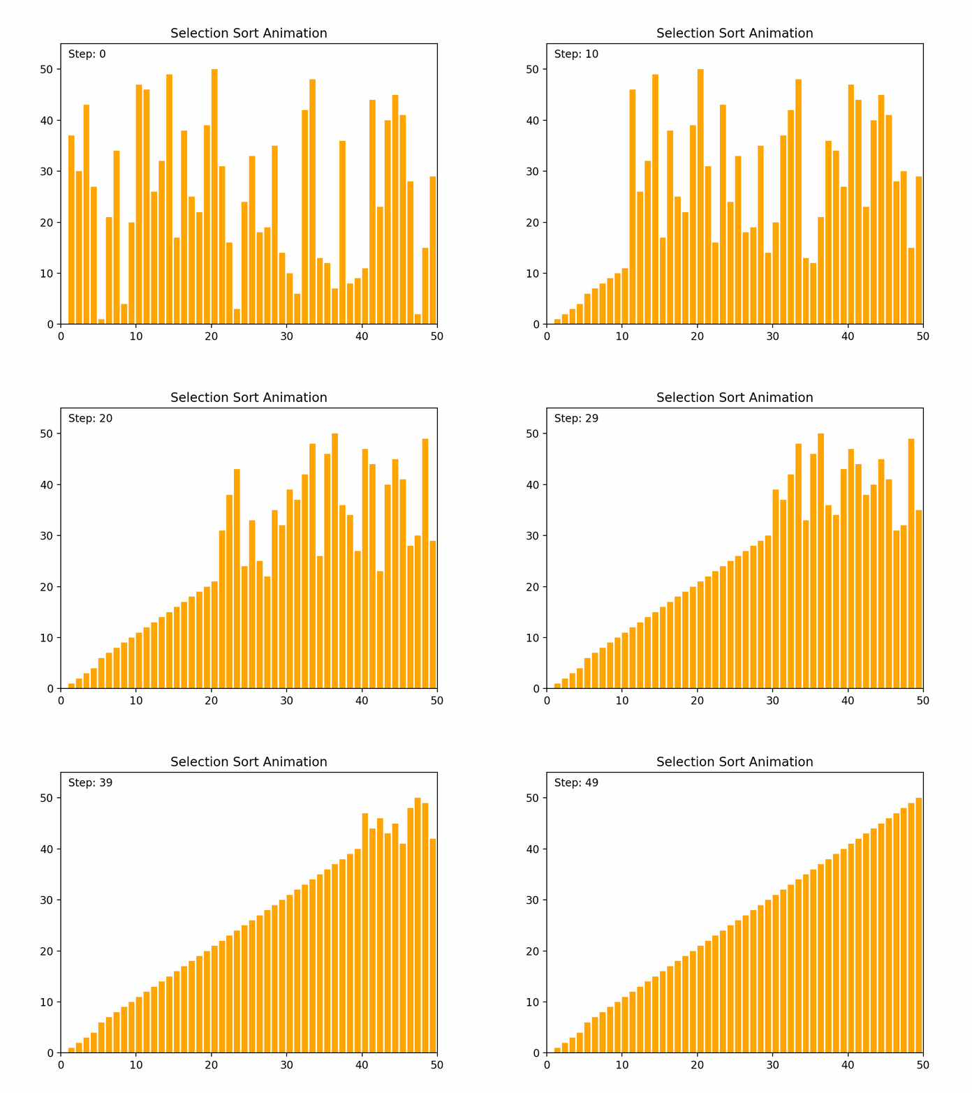
def selection_sort(arr):
frames = []
step = 0
for i in range(len(arr)):
    min_idx = i
    # Find the minimum element in remaining unsorted array
    for j in range(i+1, len(arr)):
        if arr[min_idx] > arr[j]:
            min_idx = j
    # Swap the found minimum element with the first element
    arr[i], arr[min_idx] = arr[min_idx], arr[i]
    # Append current state of array and step count to frames
    frames.append((arr.copy(), step))
    step += 1
return frames
Heap Sort
Heap sort is an efficient comparison-based sorting algorithm that uses a binary heap data structure. It is particularly noted for its good worst-case time complexity. Key Characteristics: -Time Complexity: O(n log n) for all cases (worst, average, and best), where n is the number of elements. -Space Complexity: O(1) for the in-place version, as it requires only a constant amount of additional space. -Stability: Heap sort is not stable, meaning that it does not necessarily preserve the relative order of equal elements. -Adaptability: It is not adaptive, meaning that its performance does not improve with nearly sorted lists. Algorithm Steps: 1. Build a Max Heap: Arrange the array elements into a max heap, where the largest element is at the root. 2. Extract Elements: Swap the root of the heap with the last element in the array, then reduce the heap size by one. 3. Heapify: Restore the max heap property by heapifying the root. 4. Repeat steps 2 and 3 until all elements are extracted and the array is sorted. By the end of the process, the entire list will be sorted in ascending order. Detailed Steps: 1. Build Max Heap: - Convert the array into a max heap by starting from the last non-leaf node and heapifying each node up to the root. 2. Heap Sort: - Swap the root (maximum element) with the last element of the heap. - Decrease the heap size by one. - Heapify the root to ensure the max heap property is maintained. - Repeat until the heap size is reduced to one. Heap sort's use of a binary heap ensures its efficiency and makes it suitable for large datasets.
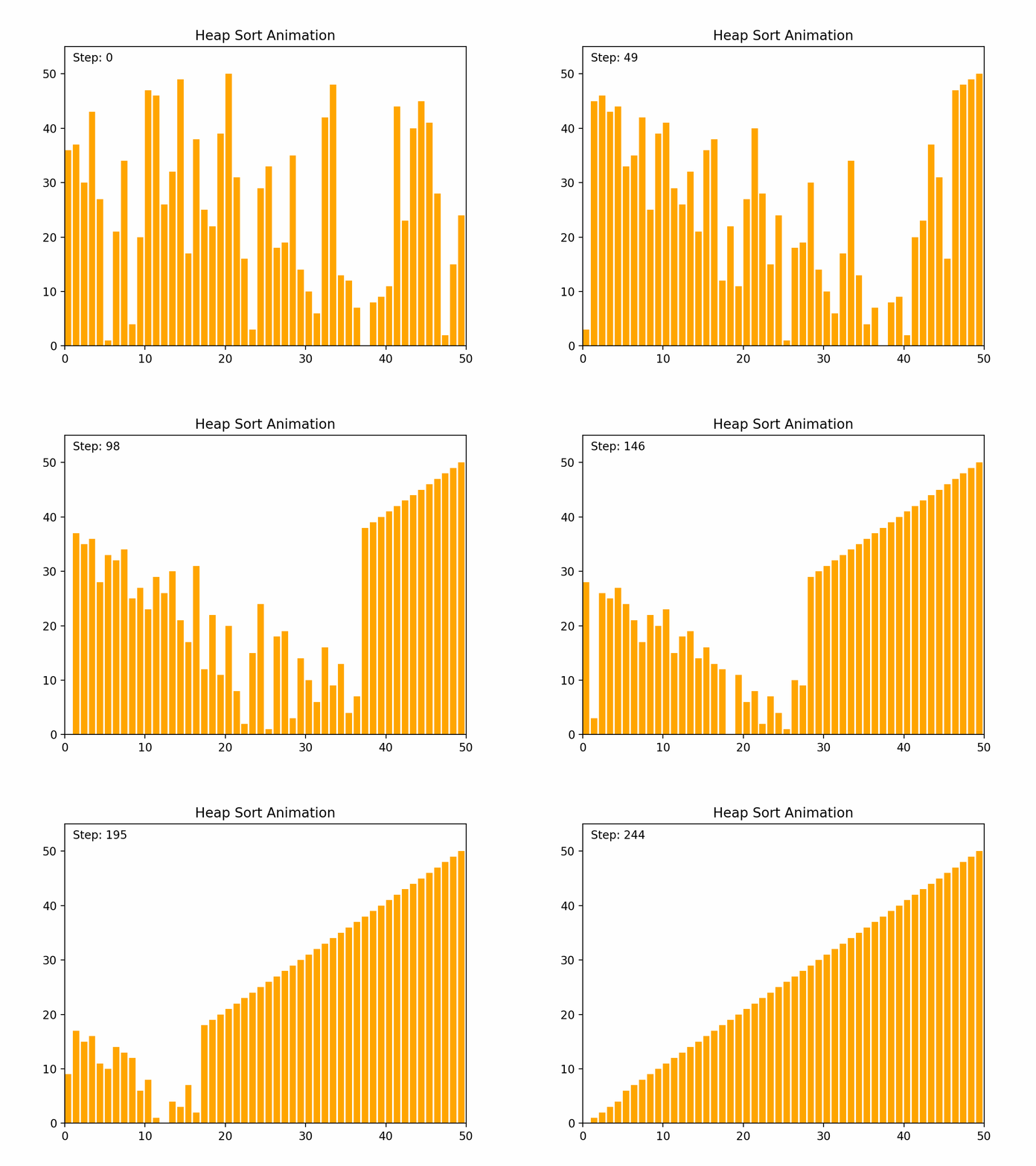
def heap_sort(arr):
frames = []
n = len(arr)
step = 0

def heapify(arr, n, i):
    nonlocal step
    largest = i  # Initialize largest as root
    l = 2 * i + 1  # left = 2*i + 1
    r = 2 * i + 2  # right = 2*i + 2

    # See if left child of root exists and is greater than root
    if l < n and arr[i] < arr[l]:
        largest = l

    # See if right child of root exists and is greater than root
    if r < n and arr[largest] < arr[r]:
        largest = r

    # Change root, if needed
    if largest != i:
        arr[i], arr[largest] = arr[largest], arr[i]
        # Append current state of array and step count to frames
        frames.append((arr.copy(), step))
        step += 1
        # Heapify the root
        heapify(arr, n, largest)

# Build a maxheap
for i in range(n // 2 - 1, -1, -1):
    heapify(arr, n, i)

# One by one extract elements
for i in range(n-1, 0, -1):
    arr[i], arr[0] = arr[0], arr[i]  # swap
    # Append current state of array and step count to frames
    frames.append((arr.copy(), step))
    step += 1
    heapify(arr, i, 0)

return frames
Quick Sort
Quick sort is a highly efficient and widely used comparison-based sorting algorithm. It employs a divide-and-conquer strategy to sort elements by partitioning the array into subarrays and recursively sorting them. Key Characteristics: - Time Complexity: - Average case: O(n log n) - Worst case: O(n²), which occurs when the pivot selection is poor (e.g., always picking the smallest or largest element). - Space Complexity: O(log n) due to the recursive stack space. - Stability: Quick sort is not stable, meaning it does not necessarily preserve the relative order of equal elements. - Adaptability: Quick sort is generally efficient for large datasets and can be optimized with good pivot selection strategies. Algorithm Steps: 1.Choose a Pivot: Select an element from the array as the pivot (commonly the first element, last element, or the median). 2.Partition: Rearrange the elements so that all elements less than the pivot are on the left, and all elements greater than the pivot are on the right. 3.Recursively Apply: Apply the same process to the left and right subarrays. Detailed Steps: 1. Partitioning: - Select a pivot element. - Rearrange the array such that elements less than the pivot are on the left and elements greater than the pivot are on the right. This may involve swapping elements. - After partitioning, the pivot is in its final position. 2. Recursion: - Recursively apply the above steps to the subarray of elements with smaller values and the subarray of elements with larger values. Example: 1. Choose a pivot element. 2. Partition the array around the pivot. 3. Recursively sort the subarrays. By repeatedly partitioning and sorting subarrays, quick sort efficiently sorts the entire array. Its performance is heavily dependent on the pivot selection method, and techniques such as randomized pivoting or the median-of-three rule can help improve its efficiency.

def quicksort(arr):
frames = []
step = 0
def _quicksort(arr, low, high):
    nonlocal step
    if low < high:
        # pi is partitioning index, arr[pi] is now at right place
        pi = partition(arr, low, high)
        # Separately sort elements before partition and after partition
        _quicksort(arr, low, pi-1)
        _quicksort(arr, pi+1, high)

def partition(arr, low, high):
    nonlocal step
    # pivot (Element to be placed at right position)
    pivot = arr[high]
    i = low - 1  # Index of smaller element
    for j in range(low, high):
        # If current element is smaller than the pivot
        if arr[j] <= pivot:
            i = i + 1
            arr[i], arr[j] = arr[j], arr[i]
            # Append current state of array and step count to frames
            frames.append((arr.copy(), step))
            step += 1
    arr[i+1], arr[high] = arr[high], arr[i+1]
    # Append current state of array and step count to frames
    frames.append((arr.copy(), step))
    step += 1
    return i + 1

_quicksort(arr, 0, len(arr) - 1)
return frames